Convergence

---

Massive amounts of care is involved with setting up simulations. We should also take great care in determining how much we can trust our simulations. This tutorial shows the user how to use the convergence submodule within biceps to determine if MCMC sampling has converged.

---

Typically, massive amounts of care is involved with setting up simulations. Thus, it is essential that we attempt to objectively uncover the validity of our simulations. Despite there being no single clear best practice to quantify MCMC sampling quality\(^{1}\), biceps.Convergence possess methods that suit our needs e.g., autocorrelation, block-averaging, bootstrapping, Jensen-Shannon divergence (JSD) and more. Previously in BICePs 1.0, trajectory convergence was measured by comparing populations and BICePs scores from sets of trajectories with varying number of steps differing by an order of magnitude. For converged results, the populations and biceps score should be similar regardless of the trajectory length.

We stress that users should check that their MCMC simulations satisfy the following items before checking convergence: 1) All states are sampled at least once over all \(\lambda\) values. The MBAR algorithm estimates conformational state populations and the states not sampled for any lambda value will be considered to have infinitely high potential energy and the corresponding predicted population will be infinite small. 2) The MCMC acceptance percentage of sample space is high. Low acceptance percentage is a sign of inefficient sampling and implies that many more steps are required to adequately sample parameter space.

import biceps

BICePs - Bayesian Inference of Conformational Populations, Version 2.0

Warning on use of the timeseries module: If the inherent timescales of the system are long compared to those being analyzed, this statistical inefficiency may be an underestimate.  The estimate presumes the use of many statistically independent samples.  Tests should be performed to assess whether this condition is satisfied.   Be cautious in the interpretation of the data.

After consideration of the latter items, the biceps.Convergence class should be used to give a statistical evaluation of convergence in MCMC trajectories. To get started, the class only requires the filename of a biceps MCMC trajectory (including its relative path) for initialization. In this step, the trajectory is read into memory and stored as the local variable convergence object C.

%matplotlib inline
C = biceps.Convergence(filename='../MP_Lambdas/results/traj_lambda0.00.npz')

To view the trajectory of 1M steps, we plot the time-series of sampled nuisance parameters (\(\sigma_{J}\), \(\sigma_{NOE}\) and \(\gamma\)).

C.plot_traces(figname="traces.pdf", xlim=(0, 1e6))

Computing the autocorrelation

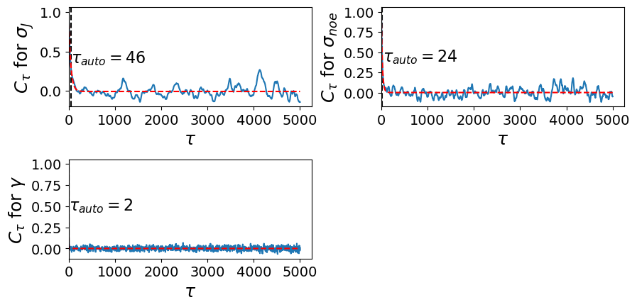
Next, we need to determine the trajectory length at which sampling becomes decorrelated. Autocorrelations curves and autocorrelation times are computed for each time-series of sampled nuisance parameters. The computed autocorrelation times for each nuisance parameter are stored in C to be used for further convergence analysis. By default, our get_autocorrelation_curves method uses an autocorrelation function (method="auto") with a window of length maxtau=10000 to compute the autocorrelation time. To obtain the autocorrelation time, we take the integral of the autocorrelation function over all lag-times \(\tau\).

Three options for the argument method are provided: block average ("block-avg"), exponential fitting ("exp") or autocorrelation function ("auto"). Each method varying in the level of statistical sophistication to compute the autocorrelation times of each nuisance parameter.

Single exponential fitting

\[f(x) = a_{0} + a_{1}*exp(-(x/\tau_{1}))\]

Computing the autocorrelation time via an exponential curve fitting is achieved by finding the best fitting of varied parameters: \(a_{0}\), \(a_{1}\) and \(\tau_{1}\). The autocorrelation time \(\tau_{auto}\)=\(\tau_{1}\) from the optimal fitting.

\begin{equation} N_{ind} = \frac{N}{1+2\tau_{auto}} \end{equation}

where \(N\) is the total number of raw samples. In practice, curve fitting method may require prior knowledge (e.g single or double exponential decay).

C.get_autocorrelation_curves(method="exp", maxtau=5000)

The functional form can also be changed from single to doubly exponential. The curve fitting method may require prior knowledge about the exponential decay. In this case, the doubly exponential decay does not apply. Below is the code that would be used:

C.exp_function = "double"
C.get_autocorrelation_curves(method="exp", maxtau=5000)

For example, a larger value of maxtau may be necessary in cases of more slowly decorrelated time series. Occasionally, negative values of \(\tau_{auto}\) may be obtained indicating the amount of data is not enough for computing autocorrelation time. Since convergence check of BICePs could be complicated, we offered multiple methods aiming for cross-validation for users to determine if the sampling achieves convergence.

Autocorrelation function \(C_{\tau}\)

\begin{equation} C\left(\theta_{t}, \theta_{t+\tau}\right) \equiv \frac{\overline{\left(\theta_{t}-\overline{\theta}\right)\left(\theta_{t+\tau}-\overline{\theta}\right)}}{s(\theta)^{2}} \Rightarrow c_{\tau} \label{eq:g} \tag{1} \end{equation}

where \(s(\theta)^{2}\) is the variance and \(c_{\tau}\) is independent of the lagtime \(\tau\). To find the proper number of lagtime (\(\tau_{auto}\)), we take integral of \(C_{\tau}\) over all lagtimes

\begin{equation} \tau_{auto} = \int C_{\tau} d \tau \label{eq:tau} \tag{2} \end{equation}

C.get_autocorrelation_curves(method="auto", maxtau=500)

Block-averaging

This approach works by partitioning a window of length maxtau into 4 blocks of equal size, then averaging the autocorrelation time for each block. Form these blocks, we can pull out the uncertainty of \(\tau_{auto}\).

C.get_autocorrelation_curves(method="block-avg-auto", maxtau=200, nblocks=5)

Please note that significant changes in the autocorrelation curve at large \(\tau\) may indicate more sampling is required and the system has not reached equilibrium. Occasionally, a negative value of \(\tau_{auto}\) may arise, which is an indication that maxtau is too small i.e., the amount of data is not enough for computing autocorrelation time. On the other hand, a slowly decorrelated time series with lots of data may also require a larger maxtau.

The JSD analysis uses the stored autocorrelation times inside the convergence object C.

Using \(\tau_{auto}\) from block averaged autocorrelations for processing (JSD distributions)

After the autocorrelation times have been stored, C.process is called to perform a series of operations including the output of plots from the resulting JSD analysis. By default, the latter method includes numerous preset arguments: nround=100 is the number of rounds of bootstrapping when computing JSDs, nfold=10 is the number of partitions in the shuffled (subsampled) trajectory, and block_avg=False specifies whether block averaging is to be used. When block_avg=True, the decorrelated time-series data gets partitioned into \(n\) blocks (nblock=5) and an average is taken over the values of greatest frequency for each block.

C.process(nblock=5, nfold=10, nround=100, savefile=False, block_avg=True, normalize=True)

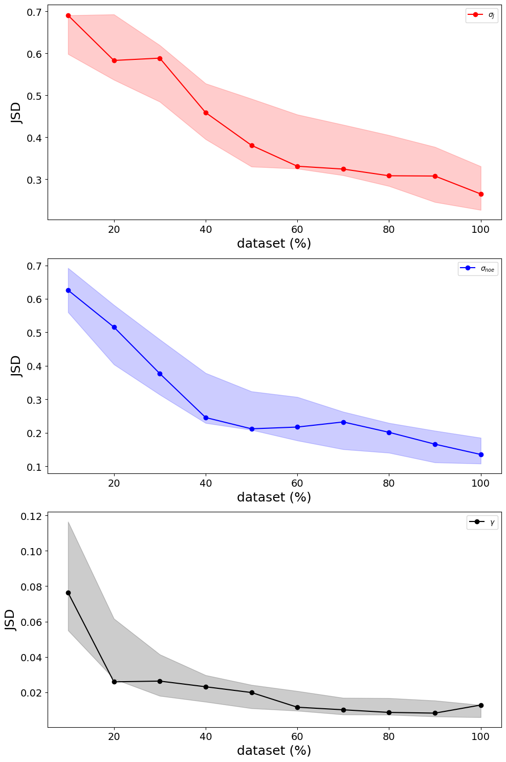
Jensen-Shannon divergence (JSD) is an improved method from Kullback-Leibler divergence and is a statistical way to measure the similarity between two probability distributions. In our convergence test, we are aiming to check if we use more data, will the distribution be different or similar to the less data which is a perfect situation that JSD calculation could be helpful. Given two sets data from BICePs sampling \(P_1\) and \(P_2\), to check if these two distribution is similar or not, we can compute the JSD as:

\begin{equation} JSD = H(P_{comb}) - {\pi_1}{H(P_1)} - {\pi_2}{H(P_2)} \label{eq:JSD_def}\tag{3} \end{equation}

where \(P_{comb}\) is the combined data (\(P_{1} \cup P_{2}\)). \(H\) is the Shannon entropy of distribution \(P_i\) and \(\pi_i\) is the weight for the probability distribution \(P_i\). Specifically, in BICePs the \(P_i\) is the distribution of sampled parameters and \({H(P_i)}\) can be computed as:

\begin{equation} {H(P_i)} = \sum -\frac{r_i}{N_i}*\ln{\frac{r_i}{N_i}} \tag{4} \end{equation}

where \(r_i\) and \(N_i\) represents sampled times of a specific parameter index and the total number of samples of the parameter, respectively. \(\pi_i\) can be computed as \(\frac{N_i}{N_{total}}\) where \(N_{total} = \sum{N_i}\). Combined together we have:

\begin{equation} JSD = \sum{(-\frac{r_{total}}{N_{total}}*\ln{\frac{r_{total}}{N_{total}}})} - \frac{N_i}{N_{total}}*\sum(-\frac{r_i}{N_i}*\ln{\frac{r_i}{N_i}}) \label{eq:JSD}\tag{5} \end{equation}

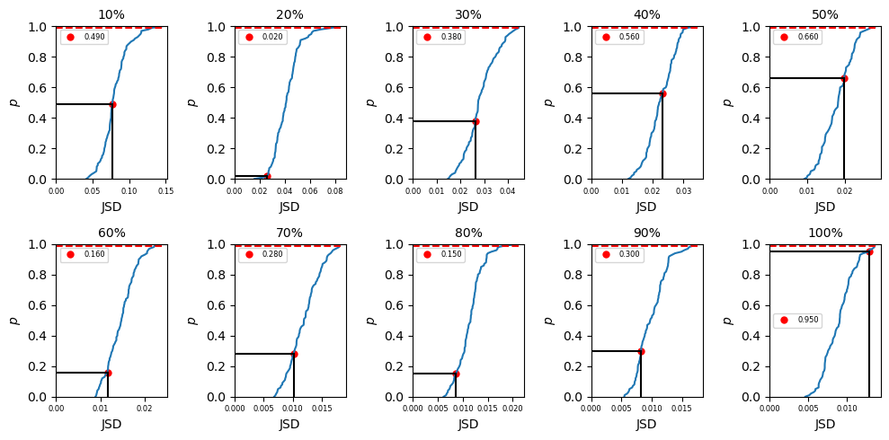
where \(i = 1, 2\) in this example. In biceps, we can import different amount of data into our JSD calculation. To do that, we may use \(p\%\) (\(p = 10,20,...100\)) data and divide the dataset (\(P_{total}\)) into two parts (the first half and second half) to get \(P_1\) and \(P_2\) in eq \ref{eq:JSD_def} and compute the JSD value (\(JSD_{single}\)) using eq \ref{eq:JSD}. 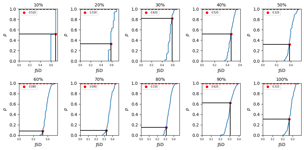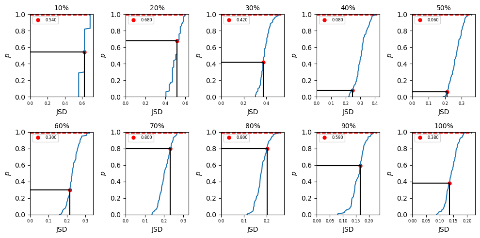Then we can randomly pick up \(N_{total}/2\) points from \(P_{total}\) as \(P_1\) (\(N_{total}\) is the total number of data after chopped) and the remaining data as \(P_2\). In this way, we are mixing the data and the computed JSD (\(JSD_{random}\)) from this mixing data should be smaller than the computed JSD from just first versus second half data. But if the dataset is completely converged, \(JSD_{single}\) and \(JSD_{random}\) should be close. Repeat mixing data \(N\) times, we shall get \(\Big\{JSD_{random}\Big\}_N\) values and a corresponded distribution. Our null hypothesis is the computed \(JSD_{single}\) is not in the distribution of \(\Big\{JSD_{random}\Big\}_N\). To test if we can accept or reject the hypothesis, we rank the \(JSD_{single}\) values in \(\Big\{JSD_{random}\Big\}_N\) in ascending order. If it is in the top 99% ranked, then we reject the hypothesis which indicates \(P_1\) and \(P_2\) no matter mixing the data or not are drawn from a mutual distribution and the data is converged. If the ranked \(JSD_{single}\) is in the last 1%, the data is not converged yet.

C.process(nblock=5, nfold=10, nround=100, savefile=False, block_avg=True, normalize=True)

In summary of the biceps.convergence class is extremely convenient and useful for objectively quantifying sampling quality. Despite there not being a one-size-fits-all approach to checking the validity of MCMC trajectories, we included an assortment of methods to check convergence. Users only need to specify the relative path and trajectory name. If desired, a method for computing the autocorrleation time can be specified. The convergence module is extremely convenient and useful for determining sufficient sampling so we can put more trust our simulations.

References

1. Grossfield, Alan, et al. “Best practices for quantification of uncertainty and sampling quality in molecular simulations [Article v1. 0].” Living journal of computational molecular science 1.1 (2018). ↩

# NOTE: The following cell is for pretty notebook rendering

from IPython.core.display import HTML
def css_styling():
    styles = open("../../../theme.css", "r").read()
    return HTML(styles)
css_styling()