Analysis

---

In this tutorial, we show the user how to instantiate the biceps.Analysis class which uses MBAR to get predicted populations of each conformational states and compute a BICePs score. We also provide a short description of the output data from analysis and embed the figures of posterior distribution of populations & nuisance parameters. Please refer to the documentation of Analysis for more specific details.

---

import biceps
import warnings
warnings.filterwarnings("ignore", category=UserWarning)
warnings.filterwarnings('ignore', category=FutureWarning)

%matplotlib inline
A = biceps.Analysis(outdir="results", nstates=100, verbose=True)
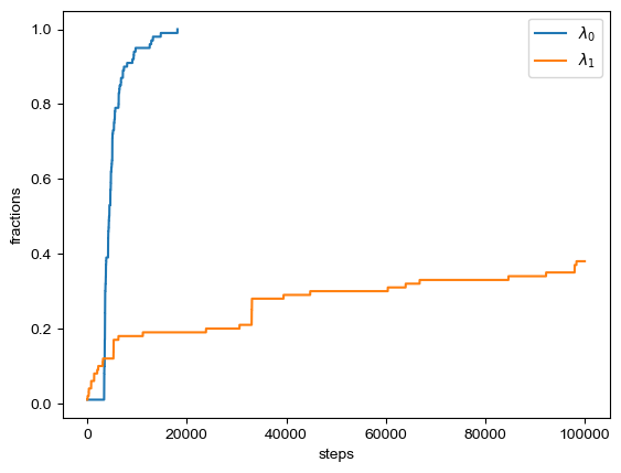
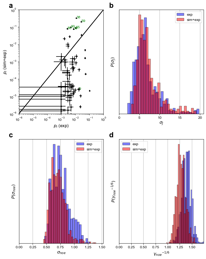
fig = A.plot(plottype="hist") # plottype="step")

Loading results/traj_lambda0.00.npz ...
Loading results/traj_lambda1.00.npz ...
not all state sampled, these states [ 0  3  4  5  8  9 11 13 14 15 16 18 19 20 21 22 23 24 25 26 27 28 29 31
 34 40 41 42 43 44 48 49 51 52 53 54 55 57 60 61 62 64 69 71 72 73 74 76
 77 78 81 82 83 86 87 88 89 95 96 97 98 99] are not sampled
Loading results/traj_lambda0.00.pkl ...
Loading results/traj_lambda1.00.pkl ...
lam = [0.0, 1.0]
nstates 100
Time for MBAR: 0.077 s
Writing results/BS.dat...
Writing results/populations.dat...
Top 10 states: [46, 85, 92, 45, 39, 80, 65, 90, 59, 38]
Top 10 populations: [0.01001833 0.0212999  0.02792732 0.03482791 0.07746092 0.07924925
 0.08826894 0.09715671 0.20440265 0.32912632]

The output files include: population information (“populations.dat”), figure of sampled parameters distribution (“BICePs.pdf”), BICePs score information (“BS.dat”), which are shown above.

Now, let’s take a look at the populations file:

There are 100 rows corresponding to 100 clustered states. 4 columns corresponding to populations of each state (row) for 2 lambda values (first 2 columns) and population change (last 2 columns).

import pandas as pd
import numpy as np
pops = np.loadtxt('results/populations.dat')
df = pd.DataFrame(pops)
df

	0	1	2	3
0	0.017975	2.496320e-05	0.004195	5.931122e-06
1	0.009977	2.292886e-05	0.003138	7.283074e-06
2	0.002693	3.068112e-04	0.001553	1.773218e-04
3	0.000990	1.008111e-05	0.000989	1.008553e-05
4	0.000000	0.000000e+00	NaN	NaN
...	...	...	...	...
95	0.006000	1.247277e-11	0.002441	5.105694e-12
96	0.000993	6.847524e-06	0.000993	6.850553e-06
97	0.004988	1.150700e-05	0.002225	5.157574e-06
98	0.004000	4.474545e-11	0.001996	2.241289e-11
99	0.002999	5.949074e-07	0.001729	3.439323e-07

100 rows × 4 columns

Conclusion

In this tutorial, the user learned how to call on the biceps.Analysis class in order to analyze the trajectory data, which automatically plots the posterior distribution of populations & nuisance parameters.

We now conclude the series of tutorials: Preparation, Restraint, PosteriorSampler and Analysis To learn more about BICePs, please check out our other examples & tutorials here.

# NOTE: The following cell is for pretty notebook rendering

from IPython.core.display import HTML
def css_styling():
    styles = open("../../../theme.css", "r").read()
    return HTML(styles)
css_styling()